Save the info states of a loon plot widget as an RDS file

l_saveStatesRDS uses saveRDS() to save the info states of a loon plot as an R object to the named file. This is helpful, for example, when using RMarkdown or some other notebooking facility to recreate an earlier saved loon plot so as to present it in the document.

l_saveStatesRDS(p, states = c("color", "active", "selected",
  "linkingKey", "linkingGroup"), file = stop("missing name of file"),
  ...)

Arguments

p	the `l_plot` object whose info states are to be saved.
states	either the logical `TRUE` or a character vector of info states to be saved. Default value `c("color", "active", "selected", "linkingKey", "linkingGroup")` consists of `n` dimensional states that are common to many `l_plot`s and which are most important to reconstruct the plot's display in any summary. If `states` is the logical `TRUE`, by `names(p)` are saved.
file	is a string giving the file name where the saved information' will be written (custom suggests this file name end in the suffix `.rds`.
...	further arguments passed to saveRDS().

Value

a list of class `l_savedStates` containing the states and their values. Also has an attribute `l_plot_class` which contains the class vector of the plot `p`

See also

l_copyStates l_info_states readRDS saveRDS

Examples

#
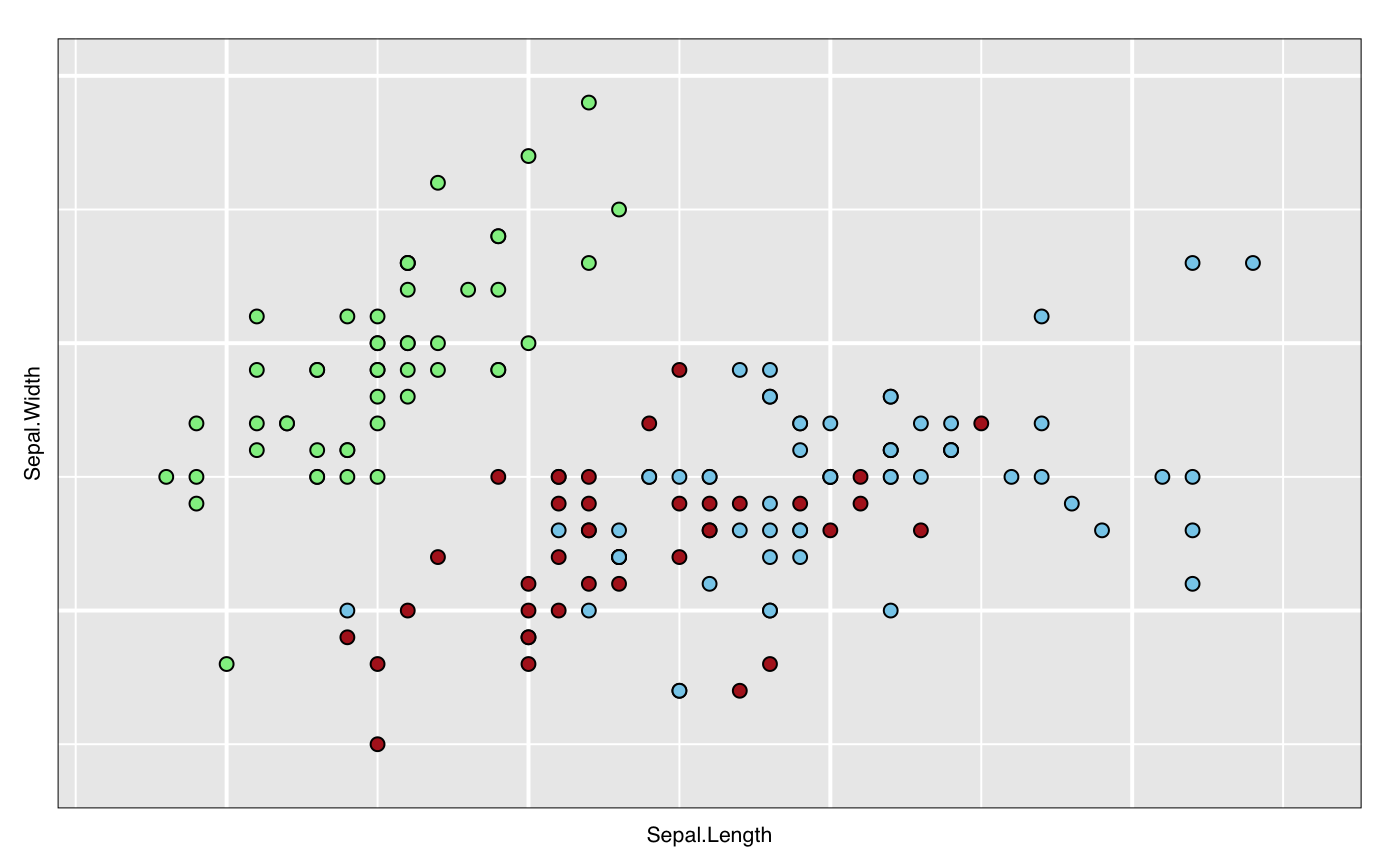
# Suppose you some plot that you created like
p <- l_plot(iris, showGuides = TRUE)
# and coloured groups by hand (using the mouse and inspector)
# so that you ended up with these colours:
p["color"] <- rep(c( "lightgreen", "firebrick","skyblue"), each = 50)
# Having determined the colours you could save them (and other states)
# in a file of your choice, here some tempfile:
myFileName <- tempfile("myPlot", fileext = ".rds")
# Save the names states of p
l_saveStatesRDS(p,
                states = c("color", "active", "selected"),
                file = myFileName)
# These can later be retrieved and used on a new plot
# (say in RMarkdown) to set the new plot's values to those
# previously determined interactively.
p_new <- l_plot(iris, showGuides = TRUE)
p_saved_info <- readRDS(myFileName)
p_new["color"] <- p_saved_info$color
# The result is that p_new looks like p did
# (after your interactive exploration)
# and can now be plotted as part of the document
plot(p_new)