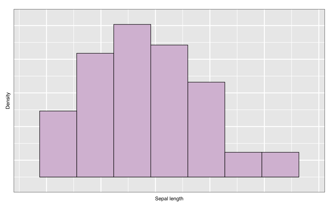
Create an interactive histogram

l_hist is a generic function for creating an interactive histogram display that can be linked with loon's other displays

l_hist(x, yshows = c("frequency", "density"), showStackedColors = TRUE,
  origin = NULL, binwidth = NULL, showBinHandle = FALSE,
  xlabel = NULL, parent = NULL, ...)

Arguments

x	vector with numerical data to perform the binning onx,
yshows	one of "frequency" (default) or "density"
showStackedColors	if TRUE (default) then bars will be coloured according to colours of the points; if FALSE, then the bars will be a uniform colour except for highlighted points.
origin	numeric scalar to define the binning origin
binwidth	a numeric scalar to specify the binwidth If NULL binwidth is set using David Scott's rule when x is numeric and and using the minumum numerical difference between factor levels when x is a factor or a character vector.
showBinHandle	If TRUE, then an interactive "bin handle" appears on the plot whose movement resets the origin and the binwidth. Default is FALSE
xlabel	label to be used on the horizontal axis. If NULL, an attempt at a meaningful label inferred from x will be made.
parent	parent widget path
...	named arguments to modify the histogram plot states

Value

widget handle

Details

Note that when changing the yshows state form 'frequency' to 'density' you might have to use l_scaleto_world to show the complete histogram in the plotting region.

For more information run: l_help("learn_R_display_hist")

See also

l_plot

Examples

h <- l_hist(iris$Sepal.Length)

names(h)
#>  [1] "linkingGroup"       "linkingKey"         "zoomX"             
#>  [4] "zoomY"              "panX"               "panY"              
#>  [7] "deltaX"             "deltaY"             "xlabel"            
#> [10] "ylabel"             "title"              "showLabels"        
#> [13] "showScales"         "swapAxes"           "showGuides"        
#> [16] "background"         "foreground"         "guidesBackground"  
#> [19] "guidelines"         "minimumMargins"     "labelMargins"      
#> [22] "scalesMargins"      "default_ylabels"    "x"                 
#> [25] "binwidth"           "origin"             "showBinHandle"     
#> [28] "yshows"             "colorStackingOrder" "showOutlines"      
#> [31] "showStackedColors"  "colorFill"          "colorOutline"      
#> [34] "color"              "selected"           "active"            
#> [37] "selectBy"           "selectionLogic"     "useLoonInspector"  
h["xlabel"] <- "Sepal length"
h["showOutlines"] <- FALSE

h["yshows"]
#> [1] "frequency"
h["yshows"] <- "density"
l_scaleto_plot(h)

h["showStackedColors"] <- TRUE
h['color'] <- iris$Species
h["showStackedColors"] <- FALSE
h["showOutlines"] <- TRUE
h["showGuides"] <- TRUE

# link another plot with the previous plot
h['linkingGroup'] <- "iris_data"
h2 <- with(iris, l_hist(Petal.Width,
                        linkingGroup="iris_data",
                        showStackedColors = TRUE))


# Get an R (grid) graphics plot of the current loon plot
plot(h)
# or with more control about grid parameters
grid.loon(h)
# or to save the grid data structure (grob) for later use
hg <- loonGrob(h)