Create a grid grob from a loon widget handle
loonGrob.RdGrid grobs are useful to create publication quality graphics.
loonGrob(target, name = NULL, gp = NULL, vp = NULL)

# S3 method for l_compound
loonGrob(target, name = NULL, gp = NULL,
  vp = NULL)

# S3 method for l_layer_graph
loonGrob(target, name = NULL, gp = NULL,
  vp = NULL)

# S3 method for l_layer_histogram
loonGrob(target, name = NULL, gp = NULL,
  vp = NULL)

# S3 method for l_layer_scatterplot
loonGrob(target, name = NULL, gp = NULL,
  vp = NULL)

# S3 method for l_navgraph
loonGrob(target, name = NULL, gp = NULL,
  vp = NULL)

# S3 method for l_navigator
loonGrob(target, name = NULL, gp = NULL,
  vp = NULL)

# S3 method for l_serialaxes
loonGrob(target, name = NULL, gp = NULL,
  vp = NULL)

# S3 method for l_ts
loonGrob(target, name = NULL, gp = NULL, vp = NULL)
Arguments
| target | either an object of class loon or a vector that specifies the
widget, layer, glyph, navigator or context completely. The widget is
specified by the widget path name (e.g. |
|---|---|
| name | a character identifier for the grob, or NULL. Used to find the grob on the display list and/or as a child of another grob. |
| gp | a gpar object, or NULL, typically the output from a call to the function gpar. This is basically a list of graphical parameter settings. |
| vp | a grid viewport object (or NULL). |
Value
a grid grob
See also
Examples
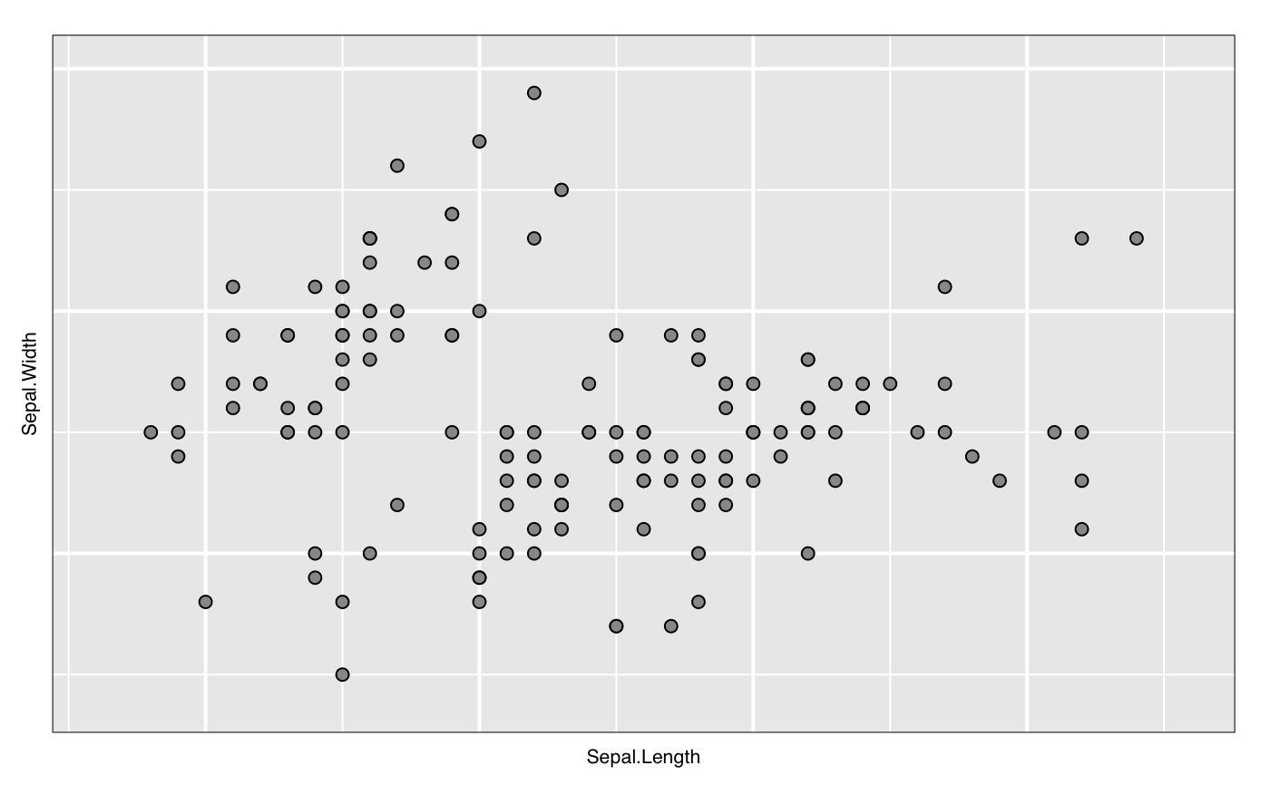
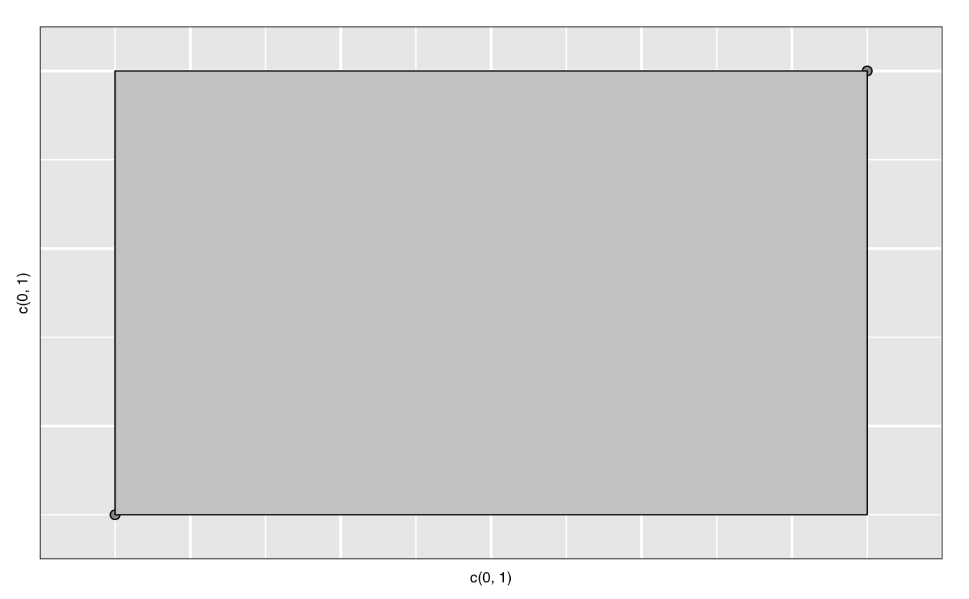
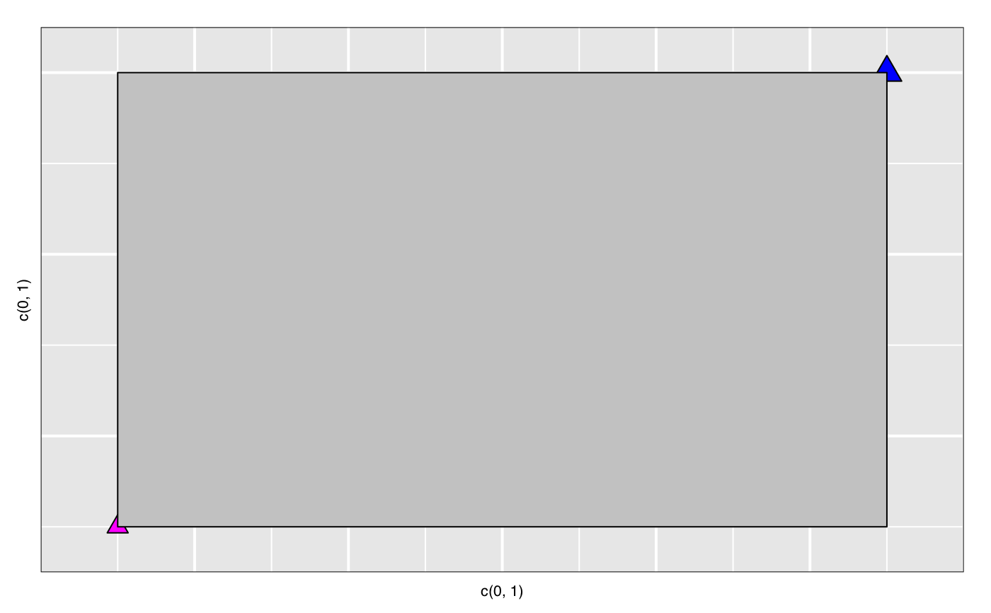
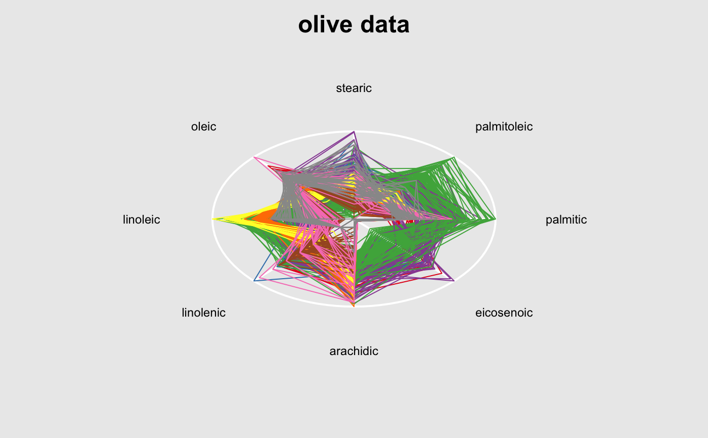
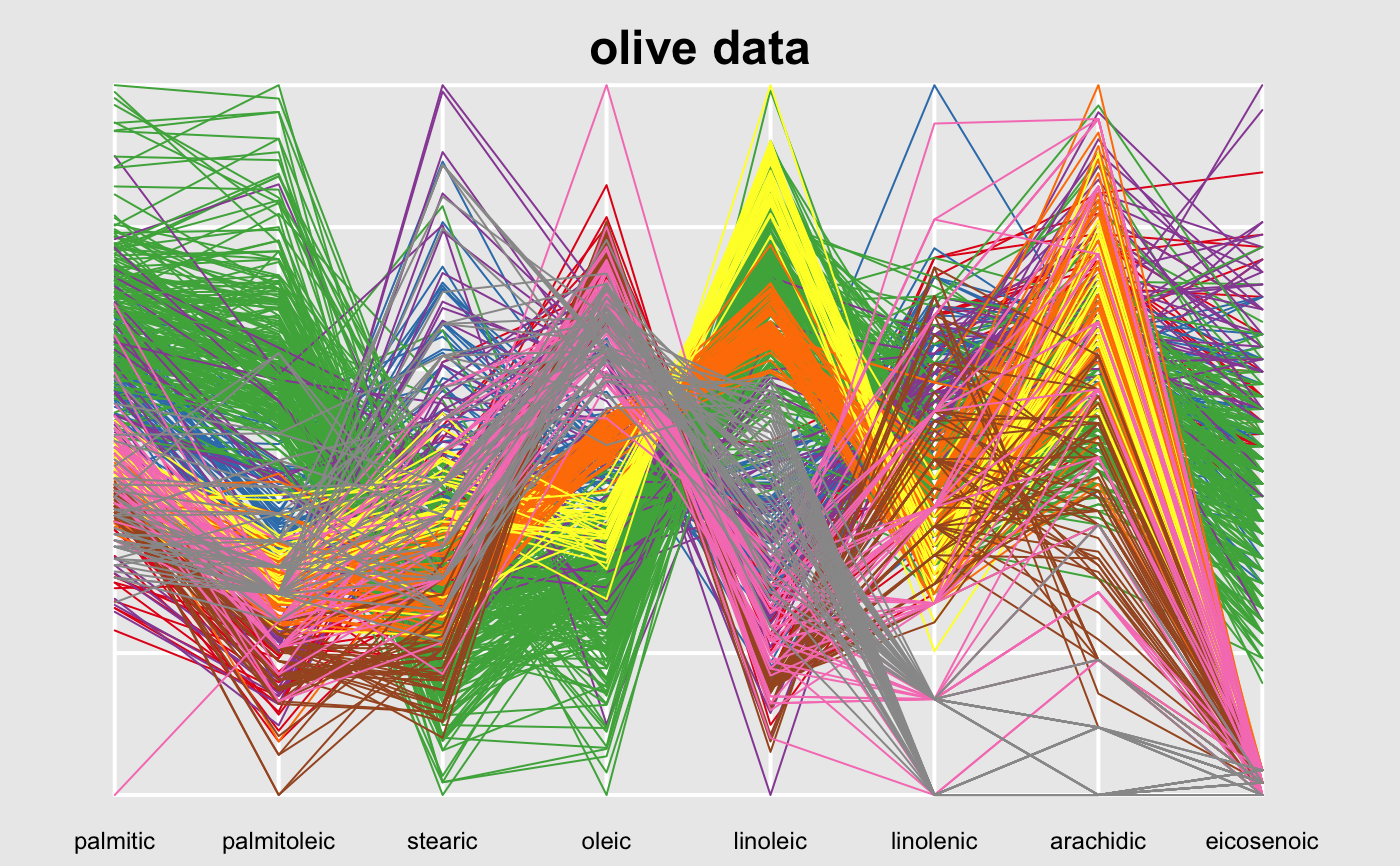
widget <- with(iris, l_plot(Sepal.Length, Sepal.Width)) lgrob <- loonGrob(widget) library(grid) grid.ls(lgrob, viewports=TRUE, fullNames=TRUE)#> gTree[GRID.gTree.75] #> gTree[l_plot] #> rect[bounding box] #> viewport[plotViewport] #> viewport[dataViewport] #> gTree[loon plot] #> gTree[labels] #> text[x label] #> text[y label] #> grob[title: textGrob arguments] #> gTree[guides] #> rect[guides background] #> lines[guidelines: xaxis (major), x = 4.5] #> lines[guidelines: xaxis (major), x = 5.5] #> lines[guidelines: xaxis (major), x = 6.5] #> lines[guidelines: xaxis (major), x = 7.5] #> lines[guidelines: xaxis (minor), x = 4] #> lines[guidelines: xaxis (minor), x = 5] #> lines[guidelines: xaxis (minor), x = 6] #> lines[guidelines: xaxis (minor), x = 7] #> lines[guidelines: xaxis (minor), x = 8] #> lines[guidelines: yaxis (major), y = 2.5] #> lines[guidelines: yaxis (major), y = 3.5] #> lines[guidelines: yaxis (major), y = 4.5] #> lines[guidelines: yaxis (minor), y = 2] #> lines[guidelines: yaxis (minor), y = 3] #> lines[guidelines: yaxis (minor), y = 4] #> gTree[axes] #> grob[x axis: xaxisGrob arguments] #> grob[y axis: yaxisGrob arguments] #> clip[clipping region] #> gTree[l_plot_layers] #> gTree[scatterplot] #> points[points: primitive glyphs with borders] #> rect[boundary rectangle] #> upViewport[2]if (FALSE) { p <- demo("l_layers", ask = FALSE)$value lgrob <- loonGrob(p) grid.newpage(); grid.draw(lgrob) p <- demo("l_glyph_sizes", ask = FALSE)$value lgrob <- loonGrob(p) grid.newpage() grid.draw(lgrob) } if (FALSE) { library(grid) ## l_pairs (scatterplot matrix) examples p <- l_pairs(iris[,-5], color=iris$Species) lgrob <- loonGrob(p) grid.newpage() grid.draw(lgrob) ## Time series decomposition examples decompose <- decompose(co2) # or decompose <- stl(co2, "per") p <- l_plot(decompose, title = "Atmospheric carbon dioxide over Mauna Loa") # To print directly use either plot(p) # or grid.loon(p) # or to save structure lgrob <- loonGrob(p) grid.newpage() grid.draw(lgrob) } if (FALSE) { ## graph examples G <- completegraph(names(iris[,-5])) LG <- linegraph(G) g <- l_graph(LG) nav0 <- l_navigator_add(g) l_configure(nav0, label = 0) con0 <- l_context_add_geodesic2d(navigator=nav0, data=iris[,-5]) nav1 <- l_navigator_add(g, from = "Sepal.Length:Petal.Width", to = "Petal.Length:Petal.Width", proportion = 0.6) l_configure(nav1, label = 1) con1 <- l_context_add_geodesic2d(navigator=nav1, data=iris[,-5]) nav2 <- l_navigator_add(g, from = "Sepal.Length:Petal.Length", to = "Sepal.Width:Petal.Length", proportion = 0.5) l_configure(nav2, label = 2) con2 <- l_context_add_geodesic2d(navigator=nav2, data=iris[,-5]) # To print directly use either plot(g) # or grid.loon(g) # or to save structure library(grid) lgrob <- loonGrob(g) grid.newpage(); grid.draw(lgrob) } if (FALSE) { ## histogram examples h <- l_hist(iris$Sepal.Length, color=iris$Species) g <- loonGrob(h) library(grid) grid.newpage(); grid.draw(g) h['showStackedColors'] <- TRUE g <- loonGrob(h) grid.newpage(); grid.draw(g) h['colorStackingOrder'] <- c("selected", unique(h['color'])) g <- loonGrob(h) grid.newpage(); grid.draw(g) h['colorStackingOrder'] <- rev(h['colorStackingOrder']) # To print directly use either plot(h) # or grid.loon(h) } ## l_plot scatterplot examples p <- l_plot(x = c(0,1), y = c(0,1)) l_layer_rectangle(p, x = c(0,1), y = c(0,1))#> loon layer "rectangle" of type rectangle of plot .l129.plot #> [1] "layer0"p['glyph'] <- "ctriangle" p['color'] <- "blue" p['size'] <- c(10, 20) p['selected'] <- c(TRUE, FALSE) g <- loonGrob(p) grid.newpage(); grid.draw(g)if (FALSE) { ## navgraph examples ng <- l_navgraph(oliveAcids, separator='-', color=olive$Area) # To print directly use either plot(ng) # or grid.loon(ng) # or to save structure lgrob <- loonGrob(ng) library(grid) grid.newpage() grid.draw(lgrob) } ## Serial axes (radial and parallel coordinate) examples s <- l_serialaxes(data=oliveAcids, color=olive$Area, title="olive data") sGrob_radial <- loonGrob(s) library(grid) grid.newpage(); grid.draw(sGrob_radial)s['axesLayout'] <- 'parallel' sGrob_parallel <- loonGrob(s) grid.newpage(); grid.draw(sGrob_parallel)if (FALSE) { ## Time series decomposition examples decompose <- decompose(co2) # or decompose <- stl(co2, "per") p <- l_plot(decompose, title = "Atmospheric carbon dioxide over Mauna Loa") # To print directly use either plot(p) # or grid.loon(p) # or to save structure lgrob <- loonGrob(p) grid.newpage() grid.draw(lgrob) }